1.1 Probability Theory and Statistics

Probability theory allows us to reason about the outcomes of random experiments. Statistical learning deals with the inverse problem: we are given the outcome of experiments, and from this we want to infer properties of the underlying mathematical structure. Suppose we have data

\[ \begin{equation} (x_1, y_1), (x_2, y_2), ..., (x_n, y_n) \end{equation} \label{eq:data} \]

where \(x_i \in \mathcal{X}\) are inputs and \(y_i \in \mathcal{Y}\) as outputs. Usually it's assumed the observations \((x_1, y_1), (x_2, y_2), ..., (x_n, y_n) \) are realizations of random variables \((X_1, Y_1), (X_2, Y_2), ..., (X_n, Y_n) \) that are i.i.d. (independent and identically distributed) with joint distribution \(P_{X,Y}\). In practice, the i.i.d. assumption is violated if distributions shift or interventions in a system occur.

We may be interested in properties of \(P_{X,Y}\), such as:

• Regression: the expectation of the output given the input \( f(x) = \mathbb{E} [Y | X = x]\), where often \(\mathcal{Y} \in \mathbb{R}\).
• A Binary Classifier: assigning each \(x\) to the class that is more likely, \[f(x) = argmax_{y \in \mathcal{Y}} P(Y=y|X=x)\] where \(\mathcal{Y} = \{\pm 1\}\)
• The density \(p_(X,Y)\) of \(P_{X,Y}\) (assuming it exists).

In practice we estimate these properties from finite data sets \(\eqref{eq:data}\) or equivalently an empirical distribution \(P^{n}_{X,Y}\).

The constitutes an inverse problem: we want to estimate a propery of an object we cannot observe (the underlying distribution), based on observations.

1.2 Learning Theory

Suppose we use the empirical distribution to infer empirical estimates \(f^n\) of functions on the underlying distribution \(f\). If the capacity of the function class is large enough that it can fit most data sets, it is not surprising that a function drawn from it would fit the data. By choosing a small capacity function class, we incorporate a priori knowledge (such as the smoothness of functions) consistent with the regularity underlying the observed data.

Machine learning proves the ability to design function classes with spectacular results. However, it is crucial that the underlying distribution does not differ between training and testing, be it by interventions or other changes.

1.3 Causal Modeling and Learning

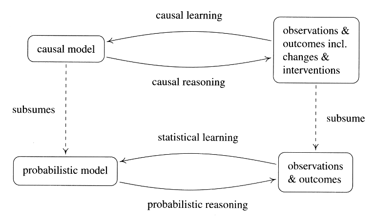
Causal modeling starts from a causal structure. A causal structure entails a probability model but contains additional information. Causal reasoning draws conclusions from a causal model, similar to how probability theory allows us to reason about the outcomes of random experiments. Causal reasoning allows us to analyze the effects of interventions and distribution changes.

Structure learning or causal discovery denote the inverse problem: inferring causal structures from empirical implications. Closely related is structure identifiability: which parts of the causaul structure can be identified from the joint distribution. The overall problem, learning the statistics as well as the causal structure, is referred to as causal learning.

We may infer the existence of causal links from statistical dependences:

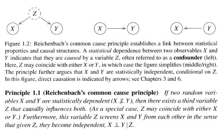
Dependences need not be from a common cause. The random variables may be conditioned on others (as in selection bias) or they only appear to be dependent.